The package bayesRecon implements several methods for probabilistic reconciliation of hierarchical time series forecasts.
The reconciliation functions are:
-
reconc_gaussian: reconciliation via conditioning of multivariate Gaussian base forecasts; this is done analytically; -
reconc_BUIS: reconciliation via conditioning of any probabilistic forecast via importance sampling; this is the recommended option for non-Gaussian base forecasts; -
reconc_MCMC: reconciliation via conditioning of discrete probabilistic forecasts via Markov Chain Monte Carlo; -
reconc_MixCond: reconciliation via conditioning of mixed hierarchies, where the upper forecasts are multivariate Gaussian and the bottom forecasts are discrete distributions; -
reconc_TDcond: reconciliation via top-down conditioning of mixed hierarchies, where the upper forecasts are multivariate Gaussian and the bottom forecasts are discrete distributions; -
reconc_t: reconciliation via conditioning with uncertain covariance of multivariate Student-t base forecasts; this is done analytically.
Getting started
The starting point for bayesRecon functions is the vignette “Get Started”. You can all find documentation in Reference section and additional vignettes in the Articles section. Finally a short example with code is provided below.
Installation
You can install the stable version on R CRAN
install.packages("bayesRecon", dependencies = TRUE)You can also install the development version from Github
# install.packages("devtools")
devtools::install_github("IDSIA/bayesRecon", build_vignettes = TRUE, dependencies = TRUE)
Getting help
If you encounter a clear bug, please file a minimal reproducible example on GitHub.
Examples
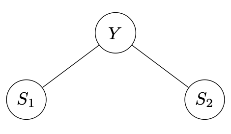
Let us consider the minimal temporal hierarchy in the figure, where the bottom variables are the two 6-monthly forecasts and the upper variable is the yearly forecast. We denote the variables for the two semesters and the year by respectively.

The hierarchy is described by the aggregation matrix A, which can be obtained using the function get_reconc_matrices.
library(bayesRecon)

rec_mat <- get_reconc_matrices(agg_levels = c(1, 2), h = 2)
A <- rec_mat$A
print(A)
#>      [,1] [,2]
#> [1,]    1    1
Example 1: Poisson base forecasts
We assume that the base forecasts are Poisson distributed, with parameters given by , , and .
lambdaS1 <- 2
lambdaS2 <- 4
lambdaY <- 9
lambdas <- c(lambdaY, lambdaS1, lambdaS2)
n_tot = length(lambdas)

base_forecasts = list()
for (i in 1:n_tot) {
  base_forecasts[[i]] = list(lambda = lambdas[i])
}
We recommend using the BUIS algorithm (Zambon et al., 2024) to sample from the reconciled distribution.
buis <- reconc_BUIS(
  A,
  base_forecasts,
  in_type = "params",
  distr = "poisson",
  num_samples = 100000,
  seed = 42
)

samples_buis <- rbind(buis$upper_rec_samples, buis$bottom_rec_samples)
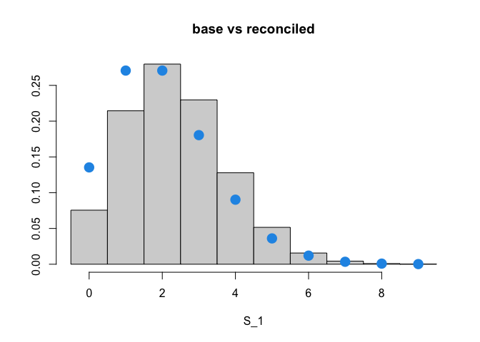
Since there is a positive incoherence in the forecasts (), the mean of the bottom reconciled forecast increases. We show below this behavior for .
reconciled_forecast_S1 <- buis$bottom_rec_samples[1,]
range_forecats <- range(reconciled_forecast_S1)
hist(
  reconciled_forecast_S1,
  breaks = seq(range_forecats[1] - 0.5, range_forecats[2] + 0.5),
  freq = F,
  xlab = "S_1",
  ylab = NULL,
  main = "base vs reconciled"
)
points(
  seq(range_forecats[1], range_forecats[2]),
  stats::dpois(seq(range_forecats[1], range_forecats[2]), lambda =
                 lambdaS1),
  pch = 16,
  col = 4,
  cex = 2
)
The blue circles represent the probability mass function of a Poisson with parameter plotted on top of the histogram of the reconciled bottom forecasts for . Note how the histogram is shifted to the right.
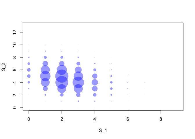
Moreover, while the base bottom forecast were assumed independent, the operation of reconciliation introduced a negative correlation between and . We can visualize it with the plot below which shows the empirical correlations between the reconciled samples of and the reconciled samples of .
AA <-
  xyTable(buis$bottom_rec_samples[1, ],
          buis$bottom_rec_samples[2, ])
plot(
  AA$x ,
  AA$y ,
  cex = AA$number * 0.001  ,
  pch = 16 ,
  col = rgb(0, 0, 1, 0.4) ,
  xlab = "S_1" ,
  ylab = "S_2" ,
  xlim = range(buis$bottom_rec_samples[1, ]) ,
  ylim = range(buis$bottom_rec_samples[2, ])
)
We also provide a function for sampling using Markov Chain Monte Carlo (Corani et al., 2023).
mcmc = reconc_MCMC(
  A,
  base_forecasts,
  distr = "poisson",
  num_samples = 30000,
  seed = 42
)

samples_mcmc <- rbind(mcmc$upper_rec_samples, mcmc$bottom_rec_samples)
Example 2: Gaussian base forecasts
We now assume that the base forecasts are Gaussian distributed, with parameters given by
- , , and ;
- , , and .
muS1 <- 2
muS2 <- 4
muY <- 9
mus <- c(muY, muS1, muS2)

sigmaS1 <- 2
sigmaS2 <- 2
sigmaY <- 3
sigmas <- c(sigmaY, sigmaS1, sigmaS2)

base_forecasts = list()
for (i in 1:n_tot) {
  base_forecasts[[i]] = list(mean = mus[[i]], sd = sigmas[[i]])
}
We use the BUIS algorithm to sample from the reconciled distribution:
buis <- reconc_BUIS(
  A,
  base_forecasts,
  in_type = "params",
  distr = "gaussian",
  num_samples = 100000,
  seed = 42
)
samples_buis <- rbind(buis$upper_rec_samples, buis$bottom_rec_samples)
buis_means <- rowMeans(samples_buis)
If the base forecasts are Gaussian, the reconciled distribution is still Gaussian and can be computed in closed form:
Sigma <- diag(sigmas ^ 2)  #transform into covariance matrix
analytic_rec <- reconc_gaussian(A,
                                base_fc_mean = mus,
                                base_fc_cov = Sigma)
analytic_means_bottom <- analytic_rec$bottom_rec_mean
analytic_means_upper <- A %*% analytic_means_bottom
analytic_means <- rbind(analytic_means_upper,analytic_means_bottom)
The base means of , , and are 9, 2, 4.
The reconciled means obtained analytically are 7.41, 2.71, 4.71, while the reconciled means obtained via BUIS are 7.41, 2.71, 4.71.
References
Carrara, C., Corani, G., Azzimonti, D., Zambon, L. (2025). Modeling the uncertainty on the covariance matrix for probabilistic forecast reconciliation. arXiv preprint arXiv:2506.19554. Available here
Corani, G., Azzimonti, D., Augusto, J.P.S.C., Zaffalon, M. (2021). Probabilistic Reconciliation of Hierarchical Forecast via Bayes’ Rule. ECML PKDD 2020. Lecture Notes in Computer Science, vol 12459. DOI
Corani, G., Azzimonti, D., Rubattu, N. (2024). Probabilistic reconciliation of count time series. International Journal of Forecasting 40 (2), 457-469. DOI
Zambon, L., Azzimonti, D. & Corani, G. (2024). Efficient probabilistic reconciliation of forecasts for real-valued and count time series. Statistics and Computing 34 (1), 21. DOI
Zambon, L., Agosto, A., Giudici, P., Corani, G. (2024). Properties of the reconciled distributions for Gaussian and count forecasts. International Journal of Forecasting 40 (4), 1438-1448. DOI
Zambon, L., Azzimonti, D., Rubattu, N., Corani, G. (2024). Probabilistic reconciliation of mixed-type hierarchical time series. Proceedings of the Fortieth Conference on Uncertainty in Artificial Intelligence, in Proceedings of Machine Learning Research 244:4078-4095. Available here.
