Reconciliation of M5 hierarchy with mixed-type forecasts
Dario Azzimonti, Lorenzo Zambon, Nicolò Rubattu, Giorgio Corani
2024-05-29
Source:vignettes/mixed_reconciliation.Rmd
mixed_reconciliation.RmdIntroduction
This vignette partially reproduces the results of Probabilistic reconciliation of mixed-type hierarchical time series (Zambon et al. 2024), published at UAI 2024 (the 40th Conference on Uncertainty in Artificial Intelligence).
In particular, we replicate the reconciliation of the one-step ahead (h=1) forecasts of one store of the M5 competition (Makridakis, Spiliotis, and Assimakopoulos 2022). Sect. 5 of the paper presents the results for 10 stores, each reconciled 14 times using rolling one-step ahead forecasts.
Data and base forecasts
The M5 competition (Makridakis, Spiliotis, and Assimakopoulos 2022) is about daily time series of sales data referring to 10 different stores. Each store has the same hierarchy: 3049 bottom time series (single items) and 11 upper time series, obtained by aggregating the items by department, product category, and store; see the figure below.

Figure 1: graph of the M5 hierarchy.
We reproduce the results of the store “CA_1”. The base forecasts (for
h=1) of the bottom and upper time series are stored in
M5_CA1_basefc, available as data in the package. The base
forecast are computed using ADAM (Svetunkov and
Boylan 2023), implemented in the R package smooth (Svetunkov 2023).
# Hierarchy composed by 3060 time series: 3049 bottom and 11 upper
n_b <- 3049
n_u <- 11
n <- n_b + n_u

# Load matrix A
A <- M5_CA1_basefc$A

# Load base forecasts:
base_fc_upper <- M5_CA1_basefc$upper
base_fc_bottom <- M5_CA1_basefc$bottom

# We will save all the results in the list rec_fc
rec_fc <- list(
  Gauss      = list(),
  Mixed_cond = list(),
  TD_cond    = list()
)
Gaussian reconciliation
We first perform Gaussian reconciliation (Gauss, Corani et al. (2021)). It assumes all forecasts
to be Gaussian, even though the bottom base forecasts are not
Gaussian.
We assume the upper base forecasts to be a multivariate Gaussian and we estimate their covariance matrix from the in-sample residuals. We assume also the bottom base forecasts to be independent Gaussians.
# Parameters of the upper base forecast distributions
mu_u <- unlist(lapply(base_fc_upper, "[[", "mu")) # upper means
# Compute the (shrinked) covariance matrix of the residuals
residuals.upper <- lapply(base_fc_upper, "[[", "residuals")
residuals.upper <- t(do.call("rbind", residuals.upper))
Sigma_u <- schaferStrimmer_cov(residuals.upper)$shrink_cov

# Parameters of the bottom base forecast distributions
mu_b <- c()
sd_b <- c()
for (fc_b in base_fc_bottom) {
  pmf <- fc_b$pmf
  mu_b <- c(mu_b, PMF_get_mean(pmf))
  sd_b <- c(sd_b, PMF_get_var(pmf)**0.5)
}
Sigma_b <- diag(sd_b**2)

# Mean and covariance matrix of the base forecasts
base_fc_mean <- c(mu_u, mu_b)
base_fc_cov <- matrix(0, nrow = n, ncol = n)
base_fc_cov[1:n_u, 1:n_u] <- Sigma_u
base_fc_cov[(n_u + 1):n, (n_u + 1):n] <- Sigma_b
We reconcile using the function reconc_gaussian(), which
takes as input:
- the summing matrix
A; - the means of the base forecast,
base_fc_mean; - the covariance of the base forecast,
base_fc_cov.
The function returns the reconciled mean and covariance for the bottom time series.
# Gaussian reconciliation
start <- Sys.time()
gauss <- reconc_gaussian(A, base_fc_mean, base_fc_cov)
stop <- Sys.time()

rec_fc$Gauss <- list(
  mu_b = gauss$bottom_rec_mean,
  Sigma_b = gauss$bottom_rec_cov,
  mu_u = A %*% gauss$bottom_rec_mean,
  Sigma_u = A %*% gauss$bottom_rec_cov %*% t(A)
)

Gauss_time <- as.double(round(difftime(stop, start, units = "secs"), 2))
cat("Time taken by Gaussian reconciliation: ", Gauss_time, "s")
#> Time taken by Gaussian reconciliation:  0.3 s
Reconciliation with mixed-conditioning
We now reconcile the forecasts using the mixed-conditioning approach
of Zambon et al. (2024), Sect. 3. The
algorithm is implemented in the function reconc_MixCond().
The function takes as input:
- the aggregation matrix
A; - the probability mass functions of the bottom base forecasts, stored
in the list
fc_bottom_4rec; - the parameters of the multivariate Gaussian distribution for the
upper variables,
fc_upper_4rec(a list withmeanandcoventries); - additional function parameters; among those note that
num_samplesspecifies the number of samples used in the internal importance sampling (IS) algorithm.
The function returns the reconciled forecasts in the form of
probability mass functions for both the upper and bottom time series.
The function parameter return_type can be changed to
samples or all to obtain the IS samples.
seed <- 1
N_samples_IS <- 5e4

# Base forecasts
fc_upper_4rec <- list(mean = mu_u, cov = Sigma_u)
fc_bottom_4rec <- lapply(base_fc_bottom, "[[", "pmf") # list of PMFs

# MixCond reconciliation
start <- Sys.time()
mix_cond <- reconc_MixCond(A, fc_bottom_4rec, fc_upper_4rec,
  bottom_in_type = "pmf",
  num_samples = N_samples_IS, return_type = "pmf", seed = seed
)
stop <- Sys.time()

rec_fc$Mixed_cond <- list(
  bottom = mix_cond$bottom_rec_pmf,
  upper  = mix_cond$upper_rec_pmf,
  ESS    = mix_cond$ESS
)

MixCond_time <- as.double(round(difftime(stop, start, units = "secs"), 2))
cat("Computational time for Mix-cond reconciliation: ", MixCond_time, "s")
#> Computational time for Mix-cond reconciliation:  10.36 s
As discussed in Zambon et al. (2024), Sect. 3, conditioning with mixed variables performs poorly in high dimensions. This is because the bottom-up distribution, built by assuming the bottom forecasts to be independent, is untenable in high dimensions. Moreover, forecasts for count time series are usually biased and their sum tends to be strongly biased; see Zambon et al. (2024), Fig. 3, for a graphical example.
Top down conditioning
Top down conditioning (TD-cond; see Zambon et
al. (2024), Sect. 4) is a more reliable approach for reconciling
mixed variables in high dimensions. The algorithm is implemented in the
function reconc_TDcond(); it takes the same arguments as
reconc_MixCond() and returns reconciled forecasts in the
same format.
N_samples_TD <- 1e4

# TDcond reconciliation
start <- Sys.time()
td <- reconc_TDcond(A, fc_bottom_4rec, fc_upper_4rec,
  bottom_in_type = "pmf", num_samples = N_samples_TD,
  return_type = "pmf", seed = seed
)
stop <- Sys.time()
The algorithm TD-cond raises a warning regarding the incoherence between the joint bottom-up and the upper base forecasts. We will see that this warning does not impact the performances of TD-cond.
Comparison
The computational time required for the Gaussian reconciliation is 0.3 seconds, Mix-cond requires 10.36 seconds and TD-cond requires 11.53 seconds.
For each time series in the hierarchy, we compute the following scores for each method:
MASE: Mean Absolute Scaled Error
MIS: Mean Interval Score
RPS: Ranked Probability Score
# Parameters for computing the scores
alpha <- 0.1 # MIS uses 90% coverage intervals
jitt <- 1e-9 # jitter for numerical stability

# Save actual values
actuals_u <- unlist(lapply(base_fc_upper, "[[", "actual"))
actuals_b <- unlist(lapply(base_fc_bottom, "[[", "actual"))
actuals <- c(actuals_u, actuals_b)

# Scaling factor for computing MASE
Q_u <- M5_CA1_basefc$Q_u
Q_b <- M5_CA1_basefc$Q_b
Q <- c(Q_u, Q_b)

# Initialize lists to save the results
mase <- list()
mis <- list()
rps <- list()
The following functions are used for computing the scores:
-
AE_pmf: compute the absolute error for a PMF; -
MIS_pmf: compute interval score for a PMF; -
RPS_pmf: compute RPS for a PMF; -
MIS_gauss: compute MIS for a Gaussian distribution.
The implementation of these functions is available in the source code of the vignette but not shown here.
# Compute scores for the base forecasts
# Upper
mu_u <- unlist(lapply(base_fc_upper, "[[", "mu"))
sd_u <- unlist(lapply(base_fc_upper, "[[", "sigma"))
mase$base[1:n_u] <- abs(mu_u - actuals_u) / Q_u
mis$base[1:n_u] <- MIS_gauss(mu_u, sd_u, actuals_u, alpha)
rps$base[1:n_u] <- scoringRules::crps(actuals_u, "norm", mean = mu_u, sd = sd_u)
# Bottom
pmfs <- lapply(base_fc_bottom, "[[", "pmf")
mase$base[(n_u + 1):n] <- mapply(AE_pmf, pmfs, actuals_b) / Q_b
mis$base[(n_u + 1):n] <- mapply(MIS_pmf, pmfs, actuals_b, MoreArgs = list(alpha = alpha))
rps$base[(n_u + 1):n] <- mapply(RPS_pmf, pmfs, actuals_b)

# Compute scores for Gauss reconciliation
mu <- c(rec_fc$Gauss$mu_u, rec_fc$Gauss$mu_b)
sd <- c(diag(rec_fc$Gauss$Sigma_u), diag(rec_fc$Gauss$Sigma_b))**0.5
sd <- sd + jitt
mase$Gauss <- abs(mu - actuals) / Q
mis$Gauss <- MIS_gauss(mu, sd, actuals, alpha)
rps$Gauss <- scoringRules::crps(actuals, "norm", mean = mu, sd = sd)

# Compute scores for Mix-cond reconciliation
pmfs <- c(rec_fc$Mixed_cond$upper, rec_fc$Mixed_cond$bottom)
mase$MixCond <- mapply(AE_pmf, pmfs, actuals) / Q
mis$MixCond <- mapply(MIS_pmf, pmfs, actuals, MoreArgs = list(alpha = alpha))
rps$MixCond <- mapply(RPS_pmf, pmfs, actuals)

# Compute scores for TD-cond reconciliation
pmfs <- c(rec_fc$TD_cond$upper, rec_fc$TD_cond$bottom)
mase$TDcond <- mapply(AE_pmf, pmfs, actuals) / Q
mis$TDcond <- mapply(MIS_pmf, pmfs, actuals, MoreArgs = list(alpha = alpha))
rps$TDcond <- mapply(RPS_pmf, pmfs, actuals)
Skill scores
We report the improvement over the base forecasts using the skill score values and averaging them across experiments. For instance, the skill score of Gauss on RPS is:
This formula is implemented in the function skill.score,
available in the source code of the vignette but not shown here.
scores <- list(
  mase = mase,
  mis = mis,
  rps = rps
)
scores_ <- names(scores)

ref_met <- "base"
methods_ <- c("Gauss", "MixCond", "TDcond")

# For each score and method we compute the skill score with respect to the base forecasts
skill_scores <- list()
for (s in scores_) {
  skill_scores[[s]] <- list()
  for (met in methods_) {
    skill_scores[[s]][["upper"]][[met]] <- skill.score(
      scores[[s]][[ref_met]][1:n_u],
      scores[[s]][[met]][1:n_u]
    )
    skill_scores[[s]][["bottom"]][[met]] <- skill.score(
      scores[[s]][[ref_met]][(n_u + 1):n],
      scores[[s]][[met]][(n_u + 1):n]
    )
  }
}
We report in the tables below the mean values for each skill score.
mean_skill_scores <- list()

for (s in scores_) {
  mean_skill_scores[[s]] <- rbind(
    data.frame(lapply(skill_scores[[s]][["upper"]], mean)),
    data.frame(lapply(skill_scores[[s]][["bottom"]], mean))
  )
  rownames(mean_skill_scores[[s]]) <- c("upper", "bottom")
}
knitr::kable(mean_skill_scores$mase, digits = 2, caption = "Mean skill score on MASE.", align = "lccc")| Gauss | MixCond | TDcond | |
|---|---|---|---|
| upper | -23.44 | -12.61 | 0.16 |
| bottom | -89.48 | -0.22 | 0.11 |
The mean MASE skill score is positive only for the TD-cond reconciliation. Both Mix-cond and Gauss achieve scores lower than the base forecasts, even if Mix-cond degrades less the base forecasts compared to Gauss.
knitr::kable(mean_skill_scores$mis, digits = 2, caption = "Mean skill score on MIS.")| Gauss | MixCond | TDcond | |
|---|---|---|---|
| upper | -66.19 | -73.49 | 1.64 |
| bottom | -36.84 | 0.21 | 2.14 |
The mean MIS score of TD-cond is slightly above that of the base forecasts. Mix-cond achieves slightly higher scores than the base forecasts only on the bottom variables. Gauss strongly degrades the base forecasts according to this metric.
knitr::kable(mean_skill_scores$rps, digits = 2, caption = "Mean skill score on RPS.")| Gauss | MixCond | TDcond | |
|---|---|---|---|
| upper | -30.69 | -24.99 | -1.3 |
| bottom | -55.62 | 2.02 | 3.9 |
The mean RPS skill score for TD-cond is positive for both upper and bottom time series. Mix-cond slightly improves the base forecasts on the bottom variables, however it degrades the upper base forecasts. Gauss strongly degrades both upper and bottom base forecasts.
Boxplots
Finally, we show the boxplots of the skill scores for each method divided in upper and bottom levels.
custom_colors <- c(
  "#a8a8e4",
  "#a9c7e4",
  "#aae4df"
)

# Boxplots of MASE skill scores
par(mfrow = c(2, 1))
boxplot(skill_scores$mase$upper,
  main = "MASE upper time series",
  col = custom_colors, ylim = c(-80, 80)
)
abline(h = 0, lty = 3)
boxplot(skill_scores$mase$bottom,
  main = "MASE bottom time series",
  col = custom_colors, ylim = c(-200, 200)
)
abline(h = 0, lty = 3)
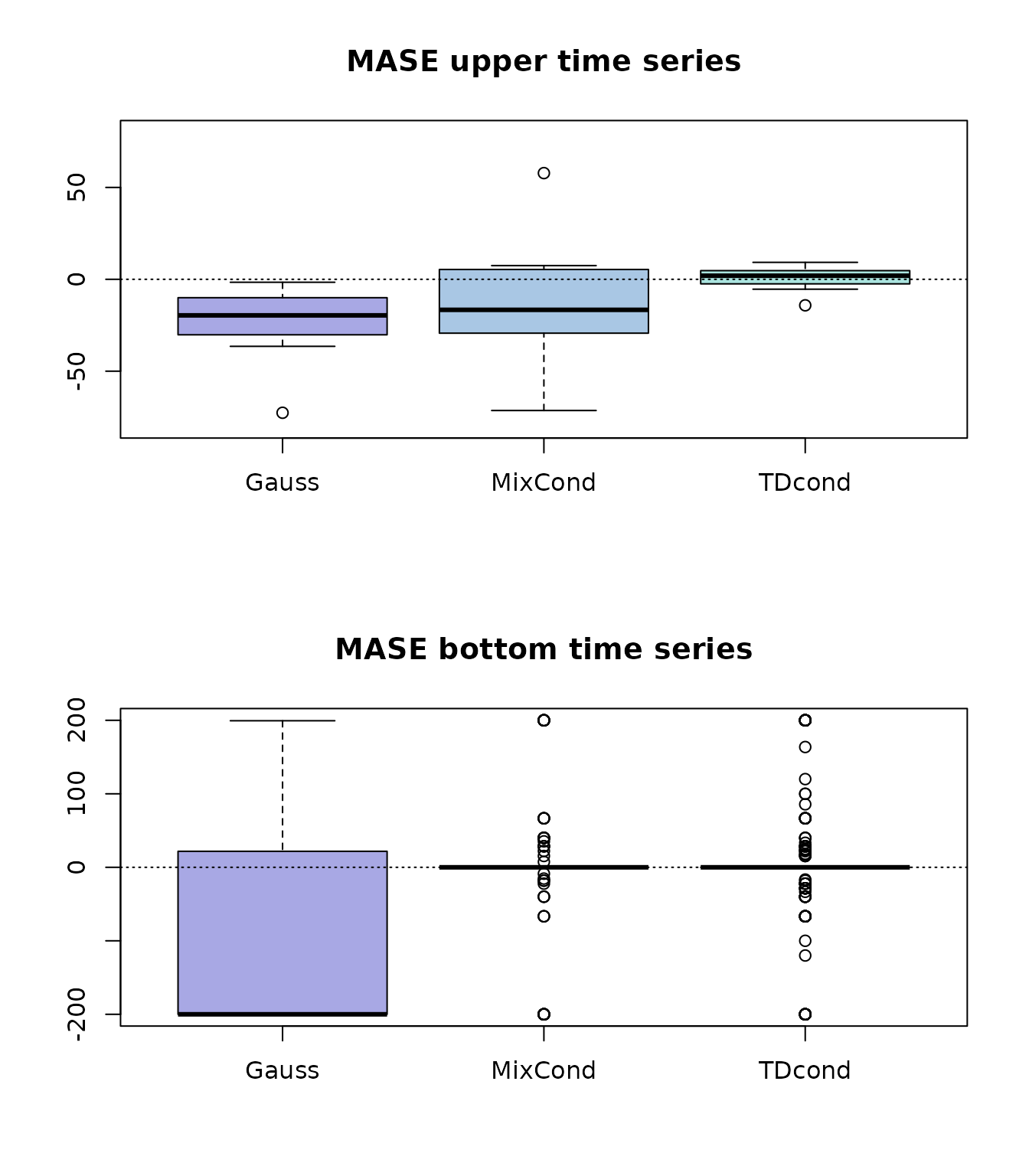
Figure 2: boxplot of MASE skill scores for upper and bottom time series.
Both Mix-cond and TD-cond do not improve the bottom MASE over the base forecasts (boxplot flattened on the value zero), however TD-cond provides a slight improvement over the upper base forecasts (boxplot over the zero line).
# Boxplots of MIS skill scores
par(mfrow = c(2, 1))
boxplot(skill_scores$mis$upper,
  main = "MIS upper time series",
  col = custom_colors, ylim = c(-150, 150)
)
abline(h = 0, lty = 3)
boxplot(skill_scores$mis$bottom,
  main = "MIS bottom time series",
  col = custom_colors, ylim = c(-200, 200)
)
abline(h = 0, lty = 3)
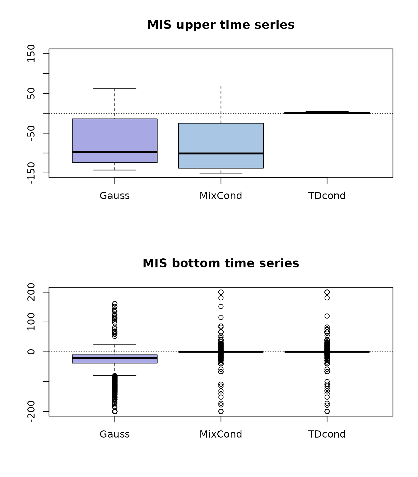
Figure 3: boxplot of MIS skill scores for upper and bottom time series.
Both Mix-cond and TD-cond do not improve nor degrade the bottom base forecasts in MIS score as shown by the small boxplots centered around zero. On the upper variables instead only TD-cond does not degrade the MIS score of the base forecasts.
# Boxplots of RPS skill scores
par(mfrow = c(2, 1))
boxplot(skill_scores$rps$upper,
  main = "RPS upper time series",
  col = custom_colors, ylim = c(-80, 80)
)
abline(h = 0, lty = 3)
boxplot(skill_scores$rps$bottom,
  main = "RPS bottom time series",
  col = custom_colors, ylim = c(-200, 200)
)
abline(h = 0, lty = 3)
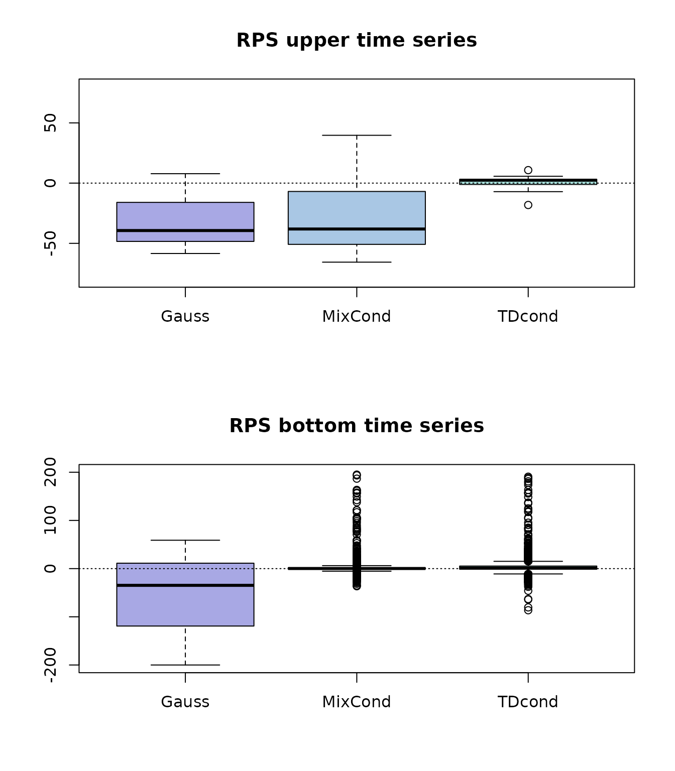
Figure 4: boxplot of RPS skill scores for upper and bottom time series.
According to RPS, TD-cond does not degrade the bottom base forecasts and improves the upper base forecasts. On the other hand both Gauss and Mix-cond strongly degrade the upper base forecasts.
Full reproducibility
The full experiment described in (Zambon et al. 2024) can be reproduced by using the code available here.